4th Blog Post
Jordan Tanley 2022-07-14
Machine Learning (woot)
What method did you find most interesting?
I think the method I found most interesting was a supervised learning method called ‘K Nearest Methods’, or KNN. This method uses the k closest observations to determine how a point should be classified. It really uses probabilities:
= proportion of k closest values that are class
= proportion of k closest values that are class
to predict which class a point belongs to (ie. the one with the highest
probability). The value of
can be hard to choose -
- too small of a
can lead to overfitting and higher variance,
- too large a
can lead to the opposite: underfitting and small variance.
To decide which value of
is best, one can use cross validatioon to use a training/testing sets.
Example
library(readr)
library(caret)
library(dplyr)
Prepare the data for kNN regression.
# read in data
heart <- read_csv("../../ST558/heart.csv")
# Create a new variable that is a factor version of the HeartDisease variable
heart$HeartDisease <- as.factor(heart$HeartDisease)
# Remove the ST_Slope variable
heart <- subset(heart, select = -c(ST_Slope))
# To use kNN we generally want to have all numeric predictors. Create dummy columns corresponding to the values of these three variables for use in our kNN fit
# use dummyVars() and predict() to create new columns. Then add these columns to our data frame and remove the original columns from which these variables were created.
dummies <- dummyVars(~ Sex + ChestPainType + RestingECG + ExerciseAngina, data = heart)
dumvars <- data.frame(predict(dummies, newdata = heart))
hearts <- cbind(heart, dumvars)
hearts <- select(hearts, -c(Sex, ChestPainType, RestingECG, ExerciseAngina))
set.seed(123)
# Split the data into a training and test set (p = .8)
# indices
train <- sample(1:nrow(hearts), size = nrow(hearts)*.8)
test <- setdiff(1:nrow(hearts), train)
# trainiing and testing subsets
heartTrain <- hearts[train, ]
heartsTest <- hearts[test, ]
# repeated 10 fold cross-validation, with the number of repeats being 3. preprocess the data by centering and scaling. set the tuneGrid so that you are considering values of k of 1, 2, 3, . . . , 40
knnfit <- train(HeartDisease ~ ., data = heartTrain, method = "knn", preProcess = c("center", "scale"),
                trControl = trainControl(method = "repeatedcv", number = 10, repeats = 3),
                tuneGrid = expand.grid(k = c(1:40)))
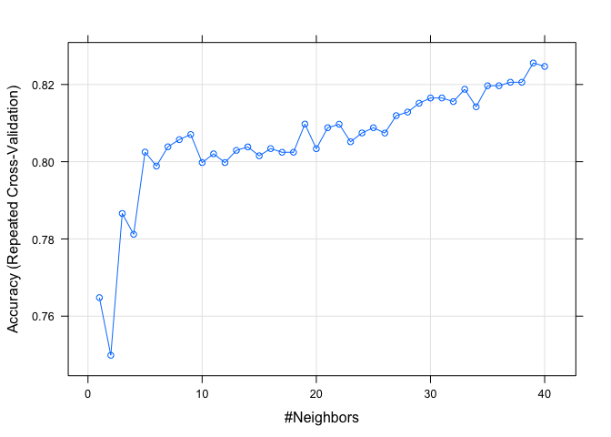
# visualize the different
plot(knnfit)

# Check how well your model does on the test set using the confusionMatrix() function
confusionMatrix(data = heartsTest$HeartDisease, reference = predict(knnfit, newdata = heartsTest))
## Confusion Matrix and Statistics
##
##           Reference
## Prediction  0  1
##          0 59 27
##          1  8 90
##
##                Accuracy : 0.8098
##                  95% CI : (0.7455, 0.8638)
##     No Information Rate : 0.6359
##     P-Value [Acc > NIR] : 2.087e-07
##
##                   Kappa : 0.6127
##
##  Mcnemar's Test P-Value : 0.002346
##
##             Sensitivity : 0.8806
##             Specificity : 0.7692
##          Pos Pred Value : 0.6860
##          Neg Pred Value : 0.9184
##              Prevalence : 0.3641
##          Detection Rate : 0.3207
##    Detection Prevalence : 0.4674
##       Balanced Accuracy : 0.8249
##
##        'Positive' Class : 0
##
From this output, we can see that according to accuracy, the model with
performed the best.