Project 1

Jordan Tanley 6/8/2022

Packages

The required packages to use the following functions and summary statistics are as follows.

knitr: Used for knitting the document
tidyverse: Used for data handling
dplyr: Helpful for data manipulation
httr: Used to access APIs
jsonlite: Aslo used to access APIs
ggplot2: Used for creating plots

API Functions

Here, I will define the function I created to access information from the PokeAPI.

`pokemonfacts`

This function has one required input:

pokemonName: The user has a choice between 10 Pokemon. These include Weedle, Butterfree, Venusaur, Bulbasaur, Squirtle, Pidgeotto, Wartortle, Blastoise, Beedrill or Charmeleon. The name must be entered as a string, (i.e. “weedle”). Capitolization does not matter here.

And several optional inputs:

base_exp: When TRUE, this option provides the base experience for the selected Pokemon. When FALSE, the value is NA.
height: When TRUE, this option provides the height for the selected Pokemon. When FALSE, the value is NA.
weight: When TRUE, this option provides the weight for the selected Pokemon. When FALSE, the value is NA.
type: When TRUE, this option provides the number of types the selected Pokemon is classified as. When FALSE, the value is NA.
color: When TRUE, this option provides the color for the selected Pokemon. When FALSE, the value is NA.
shape: When TRUE, this option provides the shape for the selected Pokemon. When FALSE, the value is NA.

When run, this function provides the selected information in the form of a data set with one row and seven columns. These collumns correspond to the name and all 6 options.

pokemonfacts <- function(pokemonName, base_exp = TRUE, height = TRUE, weight = TRUE, type = TRUE, color = TRUE, shape = TRUE){
  
  baseURL <- "https://pokeapi.co/api/v2/"
  output <- data.frame(matrix(nrow = 1))
  
  if (tolower(pokemonName) %in% "charmeleon") {
    endURL1 <- "pokemon/charmeleon"
    output$name <- "charmeleon"
    col <- GET("https://pokeapi.co/api/v2/pokemon-species/charmeleon/")
  }
  
  else if (tolower(pokemonName) %in% "pidgeotto") {
    endURL1 <- "pokemon/pidgeotto"
    output$name <- "pidgeotto"
    col <- GET("https://pokeapi.co/api/v2/pokemon-species/pidgeotto/")
  }
  
  else if (tolower(pokemonName) %in% "squirtle") {
    endURL1 <- "pokemon/squirtle"
    output$name <- "squirtle"
    col <- GET("https://pokeapi.co/api/v2/pokemon-species/squirtle/")
  }
  
  else if (tolower(pokemonName) %in% "bulbasaur") {
    endURL1 <- "pokemon/bulbasaur"
    output$name <- "bulbasaur"
    col <- GET("https://pokeapi.co/api/v2/pokemon-species/bulbasaur/")
  }
  
  
  else if (tolower(pokemonName) %in% "venusaur") {
    endURL1 <- "pokemon/venusaur"
    output$name <- "venusaur"
    col <- GET("https://pokeapi.co/api/v2/pokemon-species/venusaur/")
  }
  
  else if (tolower(pokemonName) %in% "butterfree") {
    endURL1 <- "pokemon/butterfree"
    output$name <- "butterfree"
    col <- GET("https://pokeapi.co/api/v2/pokemon-species/butterfree/")
  }
  
  else if (tolower(pokemonName) %in% "wartortle") {
    endURL1 <- "pokemon/wartortle"
    output$name <- "wartortle"
    col <- GET("https://pokeapi.co/api/v2/pokemon-species/wartortle/")
  }
  
  else if (tolower(pokemonName) %in% "weedle") {
    endURL1 <- "pokemon/weedle"
    output$name <- "weedle"
    col <- GET("https://pokeapi.co/api/v2/pokemon-species/weedle/")
  }
  
  else if (tolower(pokemonName) %in% "blastoise") {
    endURL1 <- "pokemon/blastoise"
    output$name <- "blastoise"
    col <- GET("https://pokeapi.co/api/v2/pokemon-species/blastoise/")
  }
  
  else if (tolower(pokemonName) %in% "beedrill") {
    endURL1 <- "pokemon/beedrill"
    output$name <- "beedrill"
    col <- GET("https://pokeapi.co/api/v2/pokemon-species/beedrill/")
  }
  
  else {stop("Not one of the pokemon name options. 
             Choose one of: Weedle, Butterfree, Venusaur, Bulbasaur, Squirtle, Pidgeotto, Wartortle, Blastoise, Beedrill or Charmeleon")}
  
    poke <- paste0(baseURL, endURL1) %>% GET() 
    parsed <- poke$content %>% rawToChar() %>% fromJSON()  
  
    if (base_exp) output$base_experience <- parsed$base_experience
    else {output$base_experience <- NA}
    
    if (height)   output$height <- parsed$height 
    else {output$height <- NA}
    
    if (weight) output$weight <- parsed$weight
    else {output$weight <- NA}
    
    if (type) output$types <- length(parsed$types$type$name)
    else {output$types <- NA}
    
    if (color || shape) {
      
      parsed2 <- col$content %>% rawToChar() %>% fromJSON()
      
      if (color) {output$color <- parsed2$color$name}         
      else {output$color <- NA}   
      
      if (shape) {output$shape <- parsed2$shape$name}
      else {output$shape <- NA}
      
    }
  
  Out <- subset(output, select = -1)
  
  return(Out)
}

`cleaning`

This function can be used to drop any missing values in the outputted dataframe that the previous function creates. The cases where this is useful are when the user wishes to only see a subset of the variables offered.

cleaning <- function(data){
  data %>%
    select_if(~ !any(is.na(.)))
}

Here is an example of this function at work. Originally, the dataset c has all 7 variables, with shape and color as NA. After using the cleaning() function, the NAs are dropped and the resulting dataset has 5 variables.

c <- pokemonfacts("charmeleon", shape = F, color = F)
cleaning(c)

##         name base_experience height weight types
## 1 charmeleon             142     11    190     1

`pokemon`

This function is used to combine several datasets that were created using the pokemonfacts() function. This allows the user to create a master list, or a Pokedex, of all of the pokemon that they choose to investigate. Implementation is the same as rbind(), but the name is changed to match the theme.

pokemon <- function(pokemon1, pokemon2, ...){
  out <- rbind(pokemon1, pokemon2, ...)
  return(out)
}

And that is all of the functions I created to access and use this Pokemon API! Next, I will begin some exploratory data analysis.

Exploratory Data Analysis

Next, let’s use some of the API endpoints to pull data into a dataset.

Data

The first step is to use the pokemonfacts() function to access several different endpoints. Here, I will use 10 separate endpoints, leading to 10 separate dataframes - one for each pokemon. Next, I will use the pokemon() function to concatinate the 10 datasets into one long dataset with 7 variables and 10 rows. Then, using piping from the dplyr package, I will convert the resulting dataframe to a tibble. Tibbles are helpful as they have better printing qualities than a dataframe. Finally, the resulting tibble is saved as an R object called pokedex.

# access API
c <- pokemonfacts("charmeleon")
p <- pokemonfacts("pidgeotto")
s <- pokemonfacts("squirtle")
b <- pokemonfacts("bulbasaur")
v <- pokemonfacts("venusaur")
f <- pokemonfacts("butterfree")
w <- pokemonfacts("weedle")
bl <- pokemonfacts("blastoise")
wa <- pokemonfacts("wartortle")
bee <- pokemonfacts("beedrill")
# use pokemon() function to combine all datasets into one larger one. Convert that dataframe to a tibble.
pokedex <- pokemon(s, b, p, c, v, f, w, bl, wa, bee) %>% as_tibble()
# view pokedex tibble
pokedex

## # A tibble: 10 × 7
##    name       base_experience height weight types color  shape    
##    <chr>                <int>  <int>  <int> <int> <chr>  <chr>    
##  1 squirtle                63      5     90     1 blue   upright  
##  2 bulbasaur               64      7     69     2 green  quadruped
##  3 pidgeotto              122     11    300     2 brown  wings    
##  4 charmeleon             142     11    190     1 red    upright  
##  5 venusaur               263     20   1000     2 green  quadruped
##  6 butterfree             198     11    320     2 white  bug-wings
##  7 weedle                  39      3     32     2 brown  armor    
##  8 blastoise              265     16    855     1 blue   upright  
##  9 wartortle              142     10    225     1 blue   upright  
## 10 beedrill               178     10    295     2 yellow bug-wings

For further analysis, let’s create a new variable based on the existing variables. I am interested in examining how weight classes effect their shapes, number of types, and other areas. With this in mind, lets create a size variable that classifies weight into bins of “Small”, “Medium”, or “Large”. Because of the range of weight values, I used a wider range of values for “Medium” than for the other two bins.

First, let’s create a cutoff. This is done by finding the range of values (i.e. Maximum - minimum), and then dividing by 4. I divided by 4 because I want to make the “Medium” range larger than the other bins, as stated above.
Next, we can create the new variable, size. I used the ifelse() function because a vectorized if is needed to capture all of the options for each row in the dataset.
- The “Small” category spans from the minimum value of weight to the first quartile.
- The “Medium” bin spans from the first quartile to the third quartile of weight values.
- The “Large” category spans from the third quartile to the maximum value of weight.
Finally, we can print the pokedex tibble we saved the new variable to and see our creation.

# create a cutoff by dividing the weight range by 4
cutoff <- (max(pokedex$weight) - min(pokedex$weight))/4

# use the cutoff to make bins based on weight
pokedex$size <- ifelse(pokedex$weight < cutoff, "Small", 
                  ifelse(pokedex$weight < 3*cutoff, "Medium", "Large"))
                    

pokedex

## # A tibble: 10 × 8
##    name       base_experience height weight types color  shape     size  
##    <chr>                <int>  <int>  <int> <int> <chr>  <chr>     <chr> 
##  1 squirtle                63      5     90     1 blue   upright   Small 
##  2 bulbasaur               64      7     69     2 green  quadruped Small 
##  3 pidgeotto              122     11    300     2 brown  wings     Medium
##  4 charmeleon             142     11    190     1 red    upright   Small 
##  5 venusaur               263     20   1000     2 green  quadruped Large 
##  6 butterfree             198     11    320     2 white  bug-wings Medium
##  7 weedle                  39      3     32     2 brown  armor     Small 
##  8 blastoise              265     16    855     1 blue   upright   Large 
##  9 wartortle              142     10    225     1 blue   upright   Small 
## 10 beedrill               178     10    295     2 yellow bug-wings Medium

Tables

Now, let’s create some contingency tables to futher explore this data. First, we can see some one-way tables listing the distribution of colors and shapes. It appears that the most common color is blue and the most common shape is upright for these 10 pokemon.

# one-way freq tables for color and shape
table(pokedex$color)

## 
##   blue  brown  green    red  white yellow 
##      3      2      2      1      1      1

table(pokedex$shape)

## 
##     armor bug-wings quadruped   upright     wings 
##         1         2         2         4         1

Next, we can examine some two-way contingency tables. Comparing color vs. shape, we can see that all 3 of the blue pokemon are upright in shape. Also, both of the green pokemon are quadruped. Similarly, we can look at our new variable, size, vs. shape. Ths tells us that all of the bug-wings shaped pokemon are medium in size, and the upright shaped pokemon can range greatly in size.

# contingency tables for color vs. shape and size vs. shape
table(pokedex$color, pokedex$shape)

##         
##          armor bug-wings quadruped upright wings
##   blue       0         0         0       3     0
##   brown      1         0         0       0     1
##   green      0         0         2       0     0
##   red        0         0         0       1     0
##   white      0         1         0       0     0
##   yellow     0         1         0       0     0

table(pokedex$size, pokedex$shape)

##         
##          armor bug-wings quadruped upright wings
##   Large      0         0         1       1     0
##   Medium     0         2         0       0     1
##   Small      1         0         1       3     0

Numerical Summaries

Let’s create numerical summaries for some quantitative variables at each setting of some of a categorical variable. Using piping from the dplyr package, we can group our values by color and examine a numerical summary of weight at each color level. We can see that the color blue has a very wide range of weights, with a minimum of 90 hectograms and a maximum of 855 hectograms. It is good to note that with the small size of this dataset, it is difficult to find meaningful observations when the data is split into so many groups. This is very visible when examining the variabce column. Many shape bins only have one observation, leading there to be no variance.

# group data by color. Then summarize to get min, max, median, mean, and variance of weight
pokedex %>% group_by(color) %>%
  summarize(min = min(weight), avg = mean(weight), med = median(weight), max = max(weight), var = var(weight))

## # A tibble: 6 × 6
##   color    min   avg   med   max     var
##   <chr>  <int> <dbl> <dbl> <int>   <dbl>
## 1 blue      90  390   225    855 166725 
## 2 brown     32  166   166    300  35912 
## 3 green     69  534.  534.  1000 433380.
## 4 red      190  190   190    190     NA 
## 5 white    320  320   320    320     NA 
## 6 yellow   295  295   295    295     NA

Similarly, we can group by shape and examine the weights of the pokemon in each class. We can see that quadrupeds and uprights have wide ranges in weight, both spanning just shy of 900 hectograms.

# group data by shape. Then summarize to get min, max, median, mean, and variance of weight
pokedex %>% group_by(shape) %>%
  summarize(min = min(weight), avg = mean(weight), med = median(weight), max = max(weight), var = var(weight))

## # A tibble: 5 × 6
##   shape       min   avg   med   max     var
##   <chr>     <int> <dbl> <dbl> <int>   <dbl>
## 1 armor        32   32    32     32     NA 
## 2 bug-wings   295  308.  308.   320    312.
## 3 quadruped    69  534.  534.  1000 433380.
## 4 upright      90  340   208.   855 121150 
## 5 wings       300  300   300    300     NA

Graphical Summaries

Now that we’ve got some general understanding of our data, lets visualize some of those observations we made earlier.

Fisrt up is a bar chart of the frequencies of each of the pokemon shapes. As seen earlier in the frequency table above, upright is the most common pokemon shape. In addition to the frequency of shapes, this plot also shows the frequency of total number of types that each pokemon has by shape. An interesting observation is that all four of the upright pokemon each are classified as two pokemon types. I wonder if this is the same for all upright pokemon or if it’s a mere coincidence for the ones i chose for this demonstration?

# set up plot with shape as x and color by type variable
g <- ggplot(data = pokedex, aes(x = shape, fill = as.factor(types)))
# add labels, change colors, and change label of the legend
g + geom_bar()   + labs(x = "Pokemon Shape", y = "Frequency", title = "Bar Plot of Pokemon Shapes") + scale_fill_brewer(palette = "Accent") +  guides(fill=guide_legend(title="Number of Types") ) + theme_classic()

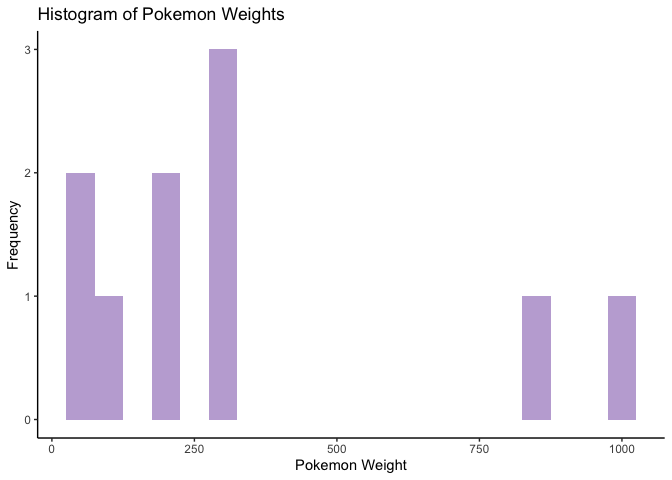
Second, we can look at a histogram of pokemon weights. This seemed fitting since the majority of our previous analysis has been on weights. Interestingly, it appears that the most common weight is around 250 hectograms, and we have a wide range from roughly 50 to 1000 hectograms.

# set up plot base with weight on x axis
g <- ggplot(data = pokedex, aes(x = weight))
# put a histogram on the plot with purple color, add labels and change theme to classic
g + geom_histogram(binwidth = 50, fill = "#c2add7") + labs(x = "Pokemon Weight", y = "Frequency", title = "Histogram of Pokemon Weights") + theme_classic()

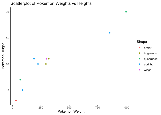
Now let’s get a little more complicated. Let’s look at a scatterplot of weight vs. height. You can see below that there is a positive linear trend between the two variables, as generally expected. As a pokemon’s weight gets larger, they also get taller. Adding another layer to this plot, we can see that the points are split up based on shape. Each color correpsonds to a different pokemon shape. One interesting thing to point out is the quadrupeds. There’s one green dot way down in the small size valeus and another in the large areas. This was expected after all of our previous analyses, but had this plot been the first thing we looked at, we would’ve wanted to look into those points further, and maybe even suspected an outlier.

# set up base plot with weight on x-axis and height on y-axis
g <- ggplot(pokedex, aes(x = weight, y = height))
# scatterplot bolor the dots by shape, add labels. Change legend title
g + geom_point(aes(color = shape))  + labs(x = "Pokemon Weight", y = "Pokemon Height", title = "Scatterplot of Pokemon Weights vs Heights")  +  guides(color=guide_legend(title="Shape")) + theme_classic() 

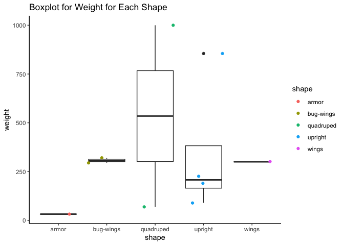
Diving a little bit deeper, we can analyze some boxplots. The first boxplot is for weights, split up by pokemon shape. This shows the range in weight for quadrupeds very dramatically. This plot also shows an outlier for the upright shaped pokemon. I will chalk this up to being due to the small size of this dataset, but it is worth mentioning.

# set up plot
g <- ggplot(pokedex, aes(x = shape, y = weight))
# white boxplots with scatterplot over them, scatter is grouped and colored by shape 
g + geom_boxplot(fill = "white") + geom_jitter(aes(group = shape, col = shape)) + labs(title = "Boxplot for Weight for Each Shape") + theme_classic() 

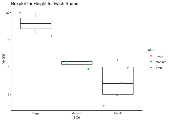
Finally, we can look at boxplots for height versus size. Since the size variable was created based on weight, it is expected that this plot will be similar to the scatterplot for weight vs. height above. And, as expected, large sized pokemon tend to be taller. The small and medium categories overlapp a bit in height, which is more interesting.

# set up plot
g <- ggplot(pokedex, aes(x = size, y = height))
# white boxplots with scatterplot over them, scatter is grouped and colored by size 
g + geom_boxplot(fill = "white") + geom_jitter(aes(group = size, col = size)) + labs(title = "Boxplot for Height for Each Shape") + theme_classic() 

As a final comment, it has appeared that the larger pokemon have a lot in common, and the contrary is true for the smaller pokemon, as there is a lot more variety among the littler guys. Gathering a larger set of data from the API could help refute or justify this claim, but that requires more time and coding.

Wrap up

Overall, APIs are great sources to use for data collection. They can be a tad confusing, but with practice and lots of useful functions, you too can create datasets, summaries, and plots with data pulled from APIs!